Simulated Sine-Wave Analysis

Frank Vanbever -- Tuesday, May 28, 2024

This is based on the scripts from Introduction to Digital Filters.

Let’s figure out the frequency response of the simplest lowpass filter:

$$ y(n) = x(n) + x(n-1),\quad n=1,2,…,N $$

We do this using simulated sine-wave analysis. This approach complements the analytical approach from the book.

First thing we need is the swanal function:

 0import numpy as np
 1from scipy.signal import lfilter
 2
 3import matplotlib.pyplot as plt
 4
 5def mod2pi(x):
 6    y = x
 7    while y >= np.pi:
 8        y = y - np.pi * 2
 9    while y < -1*np.pi:
10        y = y + np.pi * 2
11
12    return y
13
14def swanal(t,f,B,A):
15    '''Perform sine-wave analysis on filter B(z)/A/(z)'''
16    ampin = 1    # input signal amplitude
17    phasein = 0  # input signal phase
18
19    N = len(f) # Number of test frequencies
20    gains = np.zeros(N)
21    phases = np.zeros(N)
22
23    if len(A) == 1:
24        ntransient = len(B)-1
25    else:
26        error('Need to set transient response duration here')
27  
28    for k in np.arange(0,len(f)):
29        s = ampin*np.cos(2*np.pi*f[k]*t+phasein)
30        y = lfilter(B,A,s)
31        yss = y[ntransient+0:len(y)]
32        ampout = np.max(np.abs(yss))
33        peakloc = np.argmax(np.abs(yss))
34        gains[k] = ampout/ampin
35        if ampout < np.finfo(float).eps:
36            phaseout = 0
37        else:
38            # `peakloc` is an index. Matlab uses 1-based indexing whereas 
39            # Python uses 0-based indexing. 
40            sphase = 2 * np.pi * f[k] * ((peakloc+1)+ntransient-1)
41            phaseout = np.arccos(yss[peakloc]/ampout) - sphase
42            phaseout = mod2pi(phaseout)
43
44        phases[k] = phaseout - phasein
45
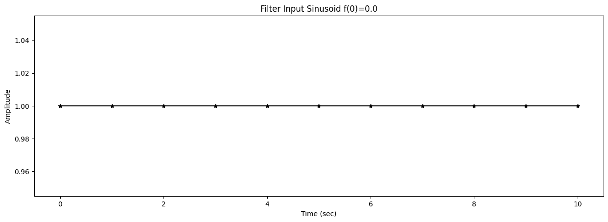
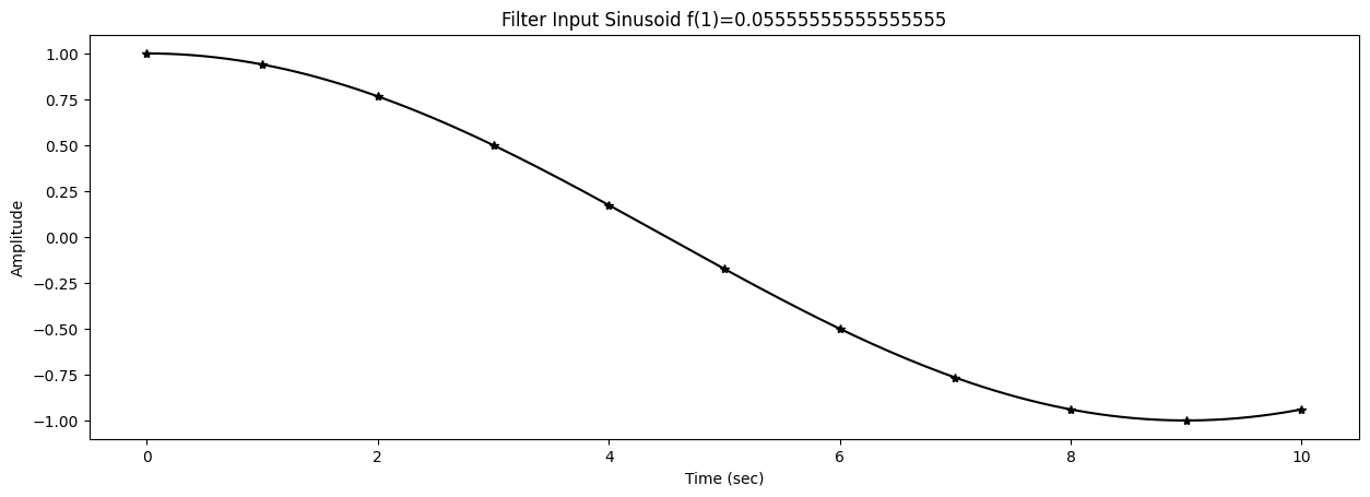
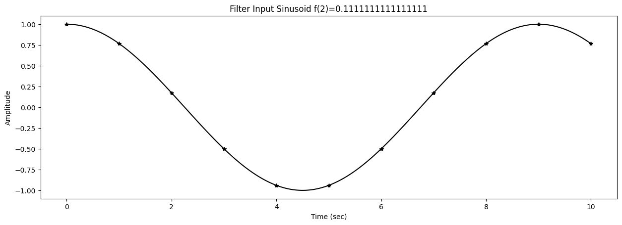
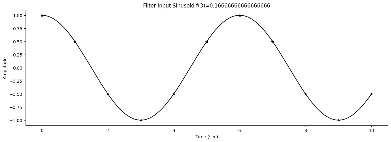
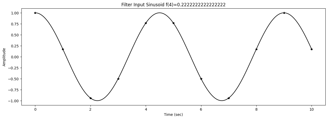
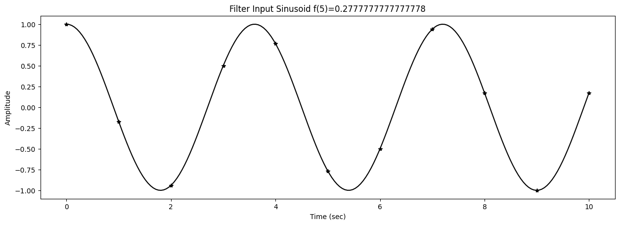
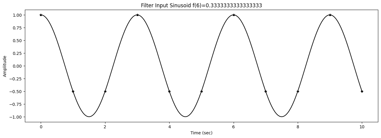
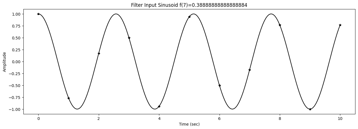
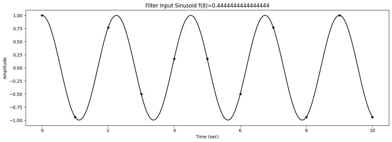
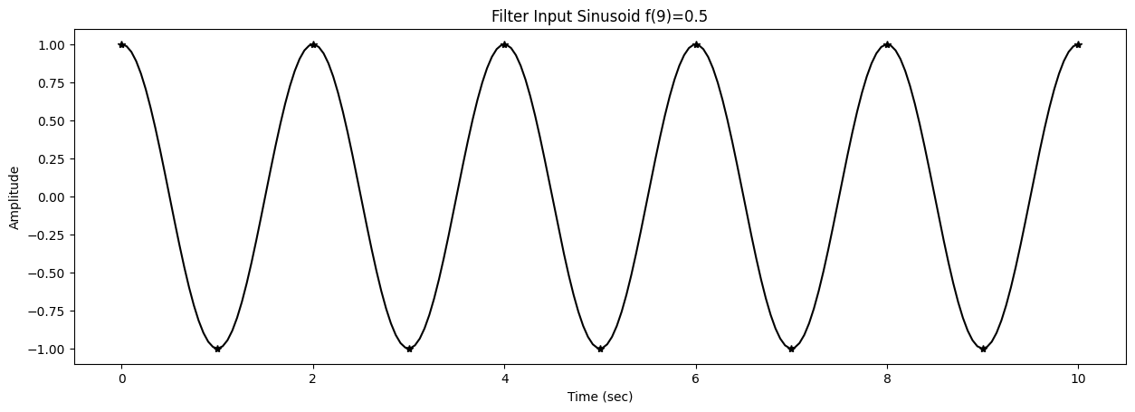
46        fig1,ax1 = plt.subplots()
47        title1 = f"Filter Input Sinusoid f({k})={f[k]}"
48        ax1.set_title(title1)
49        ax1.set_xlabel("Time (sec)")
50        ax1.set_ylabel("Amplitude")
51        ax1.plot(t,s,'*k')
52        tinterp = np.linspace(0,t[-1],num=200)
53        si = ampin*np.cos(2*np.pi*f[k]*tinterp+phasein)
54        ax1.plot(tinterp,si,'-k')
55        fig1.set_figwidth(15)
56
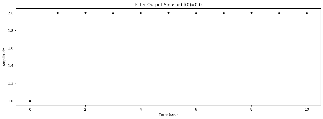
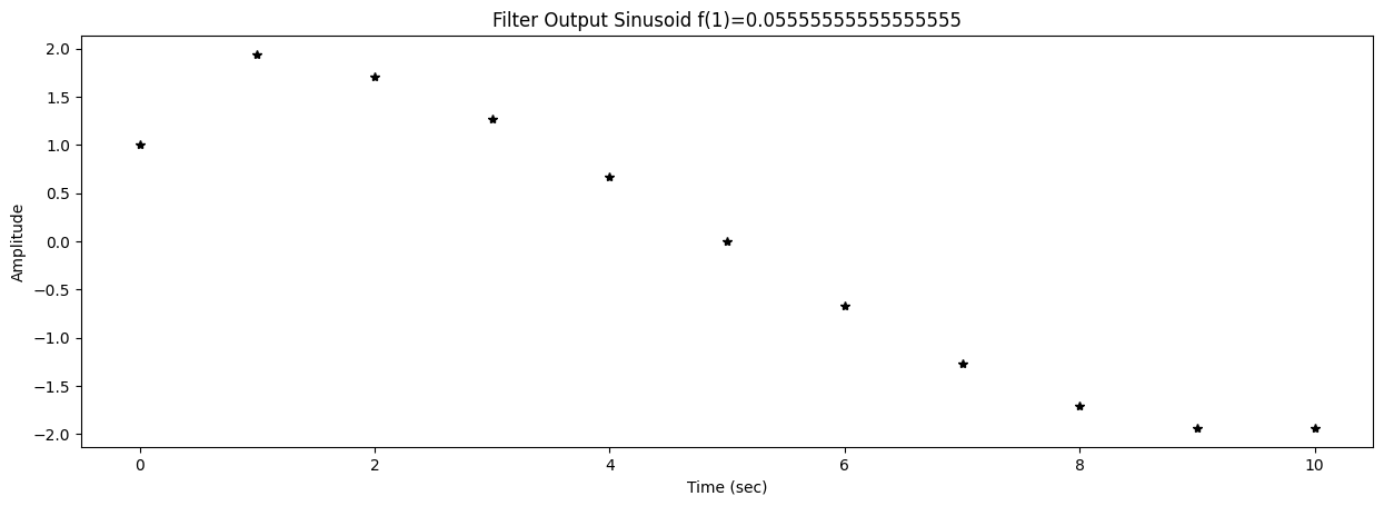
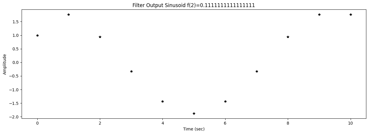
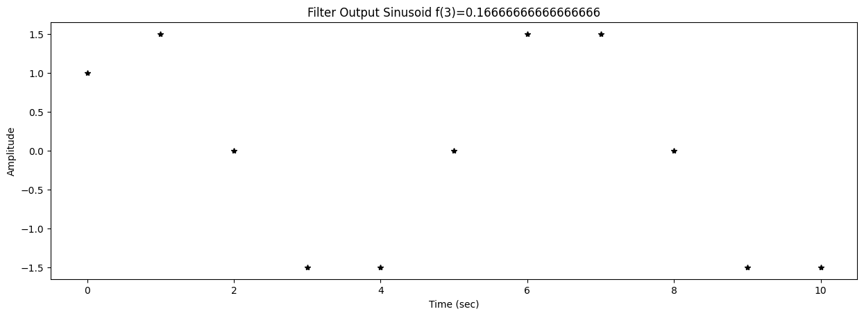
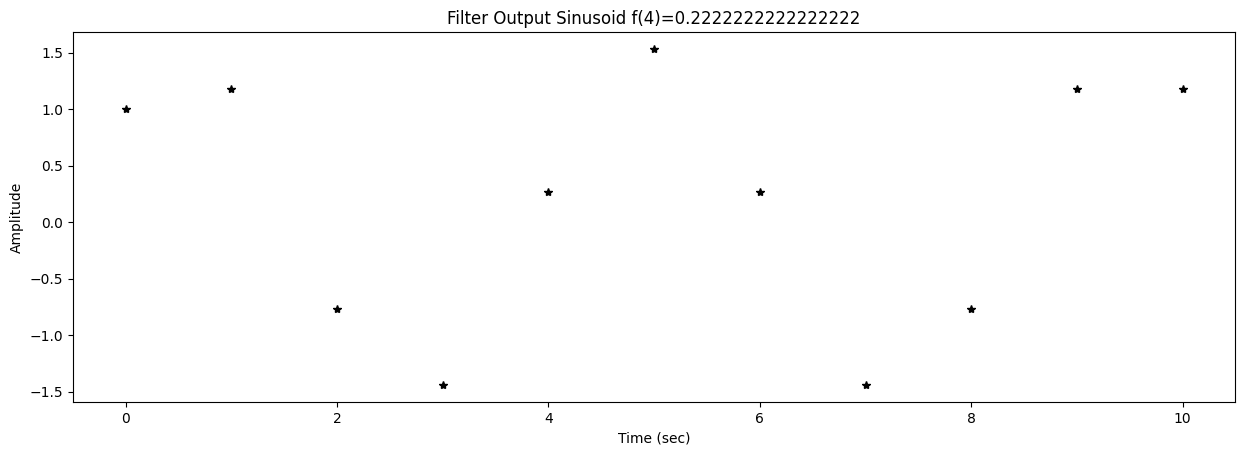
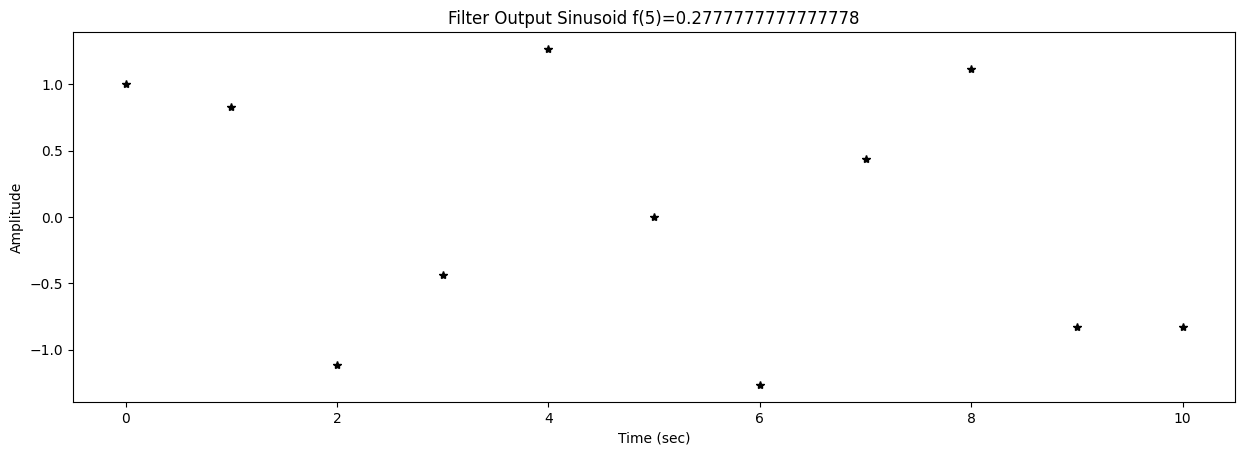
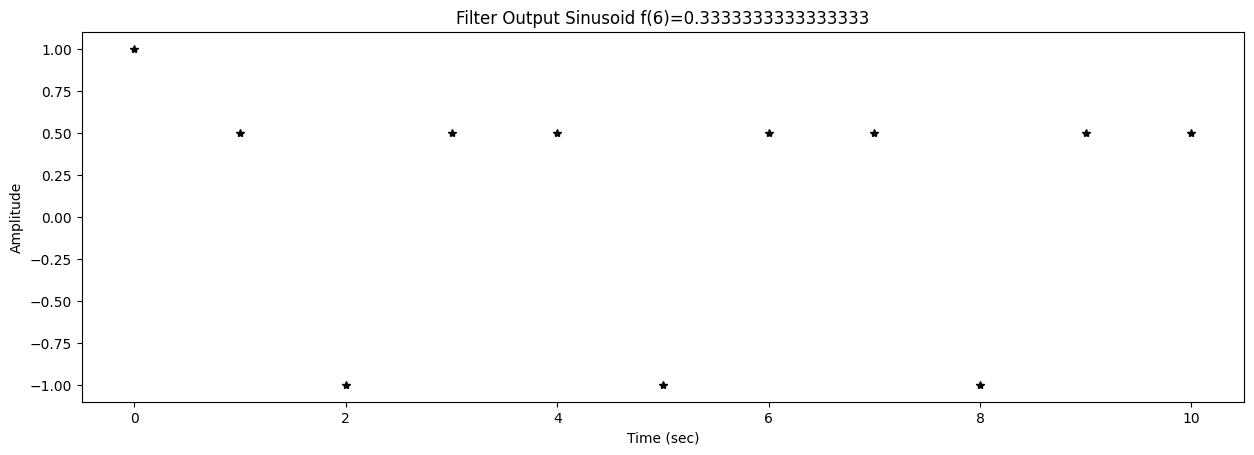
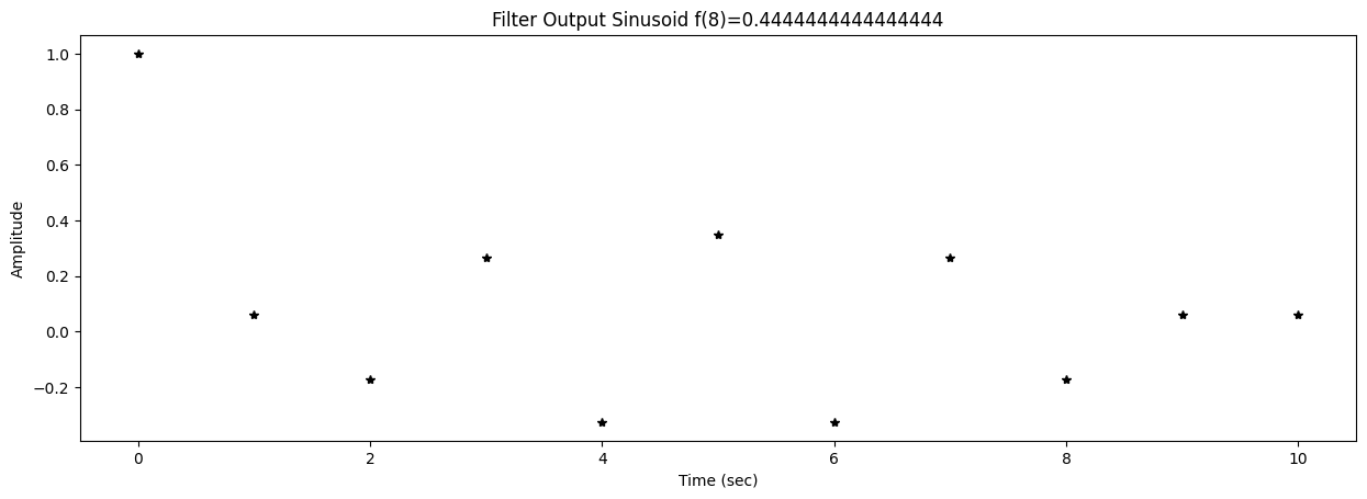
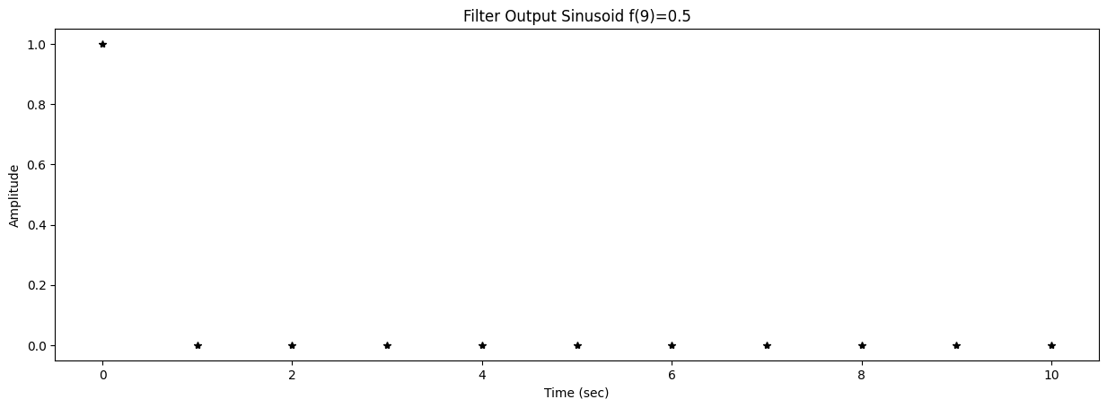
57        fig2,ax2 = plt.subplots()
58        title2 = f"Filter Output Sinusoid f({k})={f[k]}"
59        ax2.set_title(title2)
60        ax2.set_xlabel("Time (sec)")
61        ax2.set_ylabel("Amplitude")
62        ax2.plot(t,y,'*k')
63        fig2.set_figwidth(15)
64    return gains,phases

Now let’s actually use the swanal function:

 0B = [1,1]
 1A = [1]
 2
 3N = 10
 4fs = 1
 5
 6fmax = fs/2
 7df = fmax/(N-1)
 8
 9f = np.zeros(10)
10for i in range(10):
11    f[i] = i*df
12dt = 1/fs
13tmax = 10
14t = np.arange(0,tmax+1,dt)
15ampin = 1
16phasein = 0
17
18gains, phases = swanal(t, f/fs, B, A)

png

Now let’s plot these:

 0import matplotlib.pyplot as plt
 1%matplotlib inline
 2
 3def freqplot(fdata, ydata, symbol, title, xlab='Frequency', ylab='', fig=None, ax=None):
 4    if not fig or not ax:
 5        fig, ax = plt.subplots()
 6    ax.set_xlabel(xlab)
 7    ax.set_ylabel(ylab)
 8    ax.set_title(title)
 9    ax.grid()
10    ax.plot(fdata,ydata,symbol)
11    return fig, ax
12
13
14title1 = 'Amplitude Response'
15fig1, ax1 = freqplot(f, gains, '*k', title1,'Frequency (Hz)', 'Gain')
16tar = 2 * np.cos(np.pi*f/fs) # Theoretical amplitude response
17fig1, ax1 = freqplot(f, tar, '-c', title1,'Frequency (Hz)', 'Gain', fig1, ax1)
18ax1.grid()
19fig1.set_figwidth(15)
20
21
22title2 = 'Phase Response'
23tpr = -np.pi * f / fs # Theoretical Phase Response
24pscl = 1/(2*np.pi) # Convert radian phase shift to cycles
25fig2, ax2 = freqplot(f, tpr*pscl, '-c', title2, 'Frequency (Cycles)', 'Phase Shift (cycles)')
26fig2, ax2 = freqplot(f, phases*pscl, '*k', title2, 'Frequency (Cycles)', 'Phase Shift (cycles)', fig2, ax2)
27ax2.grid()
28fig2.set_figwidth(15)

png

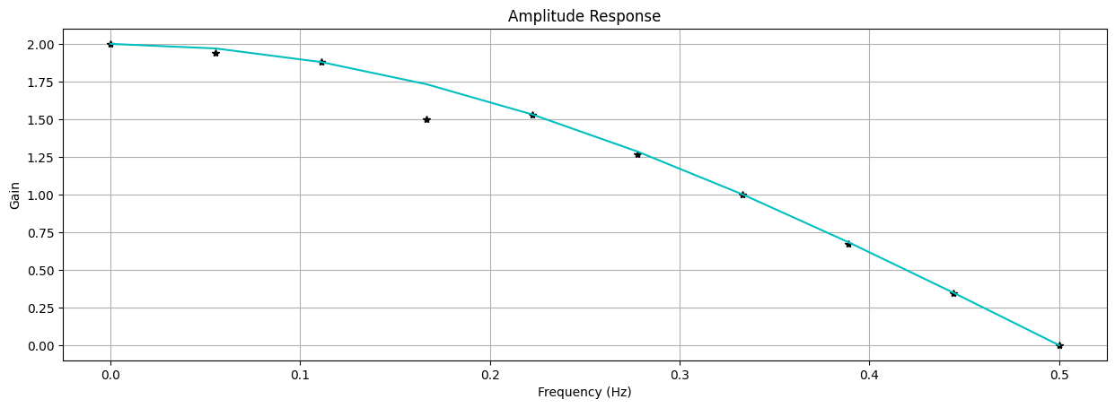
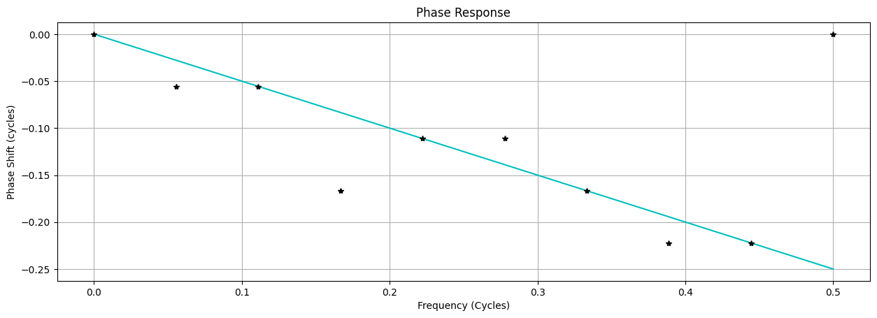
This corresponds to the graphs on the page, so yay, success! 🍾🥂

Now let’s dig deeper into what is going on here exactly.

Test sinusoids are generated with

0s = ampin * cos(2*np.pi*f[k]*t+phasein)

with:

ampin: the amplitude
f[k]: the frequency (in Hz)
phasein: the phase (in radians)

The amplitude can initially be set to 1 and the phase to 0 and if the system behaves itself (i.e. it is linear and time-invariant) then these parameters don’t matter.

0        y = lfilter(B,A,s)

applies the filter to the test sinusoid s. The coefficients in this case are:

0B = [1,1]
1A = [1]

AFAICT this is a FIR filter given that the denominator is equal to 1.

It’s best to read the book, but here is a quick summary of what this code does.

There’s 10 input sinusoids that are generated and passed through the filter. The output amplitude and phase are then estimated.

The amplitude is estimated by doing

0np.max(np.abs(yss))

This is only a rough estimation because the actual maximum is most likely located between the samples. Some interpolation would most likely solve this issue.

The phase on the other hand is estimated with the following code:

0# `peakloc` is an index. Matlab uses 1-based indexing whereas 
1            # Python uses 0-based indexing. 
2            sphase = 2 * np.pi * f[k] * ((peakloc+1)+ntransient-1)
3            phaseout = np.arccos(yss[peakloc]/ampout) - sphase
4            phaseout = mod2pi(phaseout)

sphase is the phase of the sample at the peak location in the input signal. Phaseout is then determined by finding the phase angle of the sample at the peak location in the output signal and subtracting the phase from the input to get the phase shift. mod2pi(phaseout) scales that value to the range $$ [-\pi;\pi[ $$

Once again there’s a pretty good 1-1 mapping of what Matlab/Octave provides and what Numpy/Scipy provides. One of the main sources of bugs has been the difference between 1-indexed arrays in Matlab compared to 0-indexed arrays in Python.