Pole-Zero analysis in Python with SciPy

I’m currently working on Introduction to Digital Filters By Julios O. Smit III. There’s some Matlab code for pole-zero analysis and plotting. I don’t think it makes a lot of sense to convert this to Python though, so this is me investigating what is available in SciPy.

Continuous-time Linear Systems

This part of the scipy.signal module seems to be where the interesting stuff is happening. There is an lti base class which can be instantiated with a different number of arguments:

• TransferFunction requires the numerator and denominator
• ZeroPolesGain requires us to specify the zeros, poles and gain
• StateSpace requires A, B C and D arguments

What interesting is that it’s possible to get the poles and zeros from the TransferFunction class for example, so it seems it’s possible to move between these different representations.

The difference function given in the book is the following:

$$ y(n) = x(n) + 0.5^{3}x(n-3)-0.9^{5}y(n-5) $$

if we take the Z-transform of this we get the following:

$$ Y(z) = X(z) + 0.5^{3}Z^{-3}X(Z)-0.9^{5}Z^{-5}Y(Z) $$

Given that the transfer function H(z) is given by

$$ H(z) = \frac{Y(z)}{X(z)} $$

We get the following

$$ Y(z)(1+0.9^{5}Z^{-5}) = X(z)(1+0.5^{3}Z^{-3}) $$

$$ H(z) = \frac{Y(z)}{X(z)} = \frac{1+0.5^{3}Z^{-3}}{1+0.9^{5}Z^{-5}} $$

Rewriting this in normal polynomial form by multipling with

$$ \frac{Z^{5}}{Z^{5}} $$ gives

$$ H(z) = \frac{Z^{5} + 0.5^{3}Z^{2}}{Z^{5} + 0.9^{5}} $$

Which is what we need to create our transfer function in Python:

0from scipy.signal import TransferFunction
1
2num = [1,0,0,0.5**3,0,0]
3den = [1,0,0,0,0,0.9**5]
4
5signal = TransferFunction(num, den)
6
7print(f"poles are {signal.poles}")
8print(f"zeros are{signal.zeros}")

poles are [-0.9       +0.j         -0.27811529+0.85595086j -0.27811529-0.85595086j
  0.72811529+0.52900673j  0.72811529-0.52900673j]
zeros are[-0.5 +0.j         0.25+0.4330127j  0.25-0.4330127j  0.  +0.j
  0.  +0.j       ]

These seem to correspond to the poles and zeros on figure 3.12 on this page. The next step now is to create a pole zero plot. After a bit of searching a came to the conclusion that there isn’t a pole-zero plot by default in matplotlib. There is howerver a control system library available on PyPI which supposedly provides this so let’s give it a try:

0poetry add control

 0import control as ct
 1import matplotlib.pyplot as plt
 2import numpy as np
 3
 4from matplotlib.patches import Circle
 5
 6sys = ct.tf(num,den, name="a Simple Comb Filter")
 7
 8plot_range = 1.1
 9fig1, ax1 = plt.subplots(1)
10ax1.set_title("A pole-zero plot of a Simple Comb Filter")
11ax1.set_xlim(-plot_range,plot_range)
12ax1.set_ylim(-plot_range,plot_range)
13
14circle = Circle((0,0),1,fill=False,linestyle="--")
15
16ax1.add_patch(circle)
17ax1.set_aspect('equal')
18
19ticks = np.arange(-1,1.1,0.2)
20ax1.set_xticks(ticks)
21ax1.set_yticks(ticks)
22
23ax1.grid()
24
25ct.pole_zero_plot(sys, ax=ax1)

array([[list([<matplotlib.lines.Line2D object at 0x7d3087af2e70>]),
        list([<matplotlib.lines.Line2D object at 0x7d3087af3410>])]],
      dtype=object)

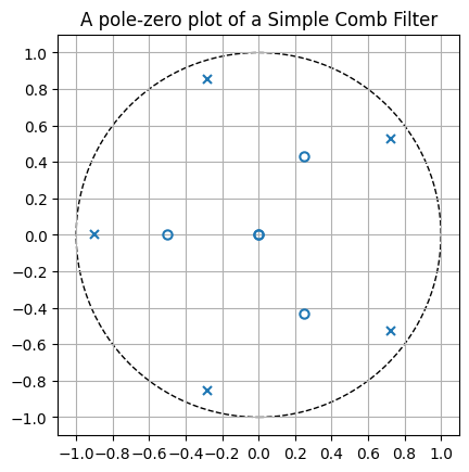
This looks quite a bit like the plot from the book. It required quite a bit of masaging, and honestly I’m not sure if it makes a lot of sense to include python-control as a dependency just to have a plot like this, maybe I should just build something on top of matplotlib myself. On the other hand, the scipy.signal makes all of these calculations a breeze so that’s definitely something for the toolbox!