Envelope Filter Model in Python
One of my goals is to code up an Envelope Filter DSP effect for bass guitar. I’ve been reading Audio Effects by Reiss & Andrew P. McPherson and I’ve gotten to the description of a wah effect with the filter controlled by an envelope follower in chapter 4. That should be enough to get a prototype implementation started in Python.
I’ll need a few things:
- A resonant low-pass filter
- An envelope follower.
I’ll do those in order.
Resonant Low-Pass filter
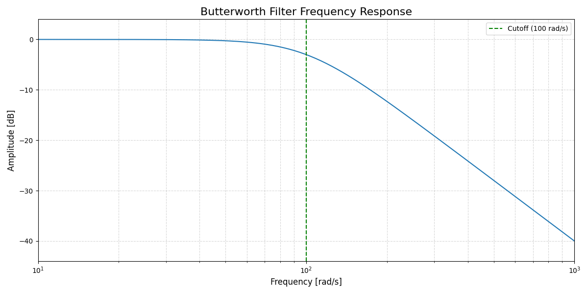
I need a filter that has a nice big resonance at the cutoff frequency. I think it would also be beneficial to not have too much (or any) ripple in the passband of the filter. Let’s have a look at the scipy toolbox.
If you look at the different types of filters available then a butterworth filter seems like it would be a good choice to start from given that it does not have any ripple in the passband. We’ll have to introduce the resonance some way though.
Let’s first get our imports out of the way:
0from scipy import signal
1import matplotlib.pyplot as plt
2import numpy as np
Now let’s start designing a filter:
 0%matplotlib ipympl
 1
 2cutoff = 100
 3b, a = signal.butter(2, cutoff, 'low', analog=True)
 4w, h = signal.freqs(b, a)
 5plt.semilogx(w, 20 * np.log10(abs(h)))
 6plt.title('Butterworth filter frequency response')
 7plt.xlabel('Frequency [rad/s]')
 8plt.ylabel('Amplitude [dB]')
 9plt.margins(0, 0.1)
10plt.grid(which='both', axis='both')
11plt.axvline(cutoff, color='green')
The filter design toolbox in Scipy seeminly does not support my use case of designing a resonant filter. I need some kind of biquad IIR filter where I have more control over the design. There seems to be a project on Pypi which does this: python-biquad. Alternatively I can do my own implementation using the audio equalizer coockbock formulae by Robert Bristow-Johnson. A low-pass filter with controls is given by:
$$ H(s) = \frac{1}{s^{2}+\frac{s}{Q}+1} $$ $$ b_{0} = \frac{1 - cos(\omega_{0})}{2} $$ $$ b_{1} = 1 - cos(\omega_{0}) $$ $$ b_{2} = \frac{1 - cos(\omega_{0})}{2} $$ $$ a_{0} = 1 + \alpha $$ $$ a_{1} = -2cos(\omega_{0}) $$ $$ a_{2} = 1 - \alpha $$
With the parameters:
$$ \omega_{0} = 2 \pi \frac{f_{0}}{F_{s}} $$
the angular frequency and
$$ \alpha = \frac{sin(\omega_{0})}{2Q} $$
 0
 1cutoff = 100
 2Fs = 48000
 3w0 = 2 * np.pi * cutoff/Fs
 4
 5Q = 10
 6alpha = np.sin(w0)/(2*Q)
 7
 8
 9b0 = (1 - np.cos(w0))/2
10b1 = 1 - np.cos(w0)
11b2 = b0
12
13a0 = 1 + alpha
14a1 = -2 * np.cos(w0)
15a2 = 1 - alpha
16
17num = [b0, b1, b2]
18den = [a0, a1, a2]
19
20w, h = signal.freqz(num, den, fs=Fs)
21
22fig1, ax1 = plt.subplots()
23ax1.set_title(f"Wah filter frequency response")
24ax1.axvline(cutoff, color='black', linestyle=':')
25ax1.semilogx(w, 20 * np.log10(abs(h)), 'C0')
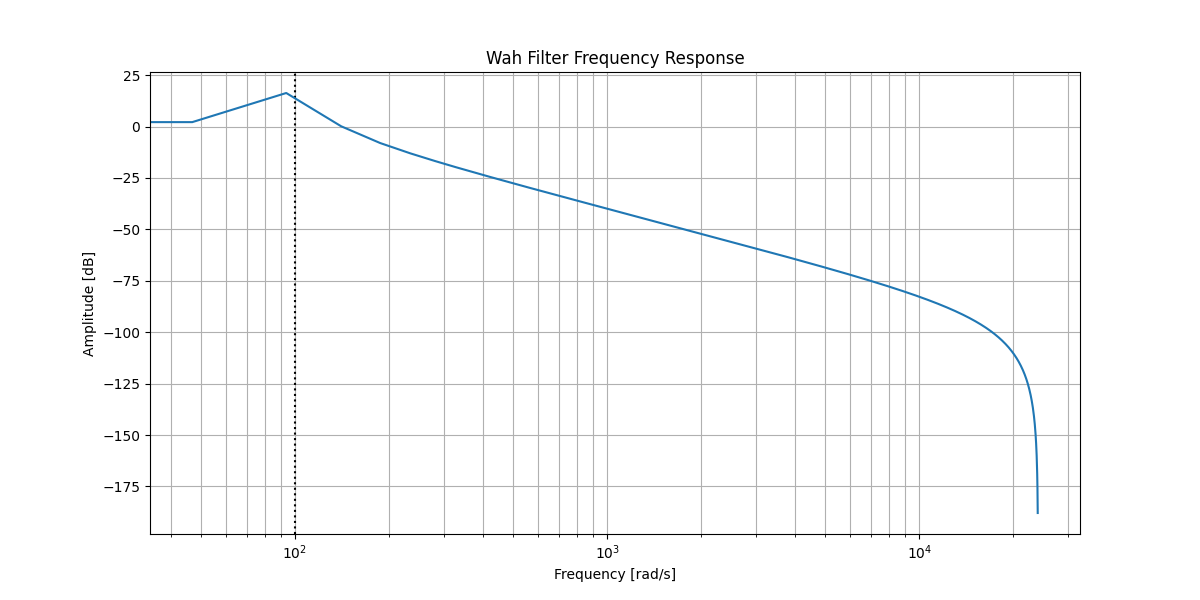
That looks like a resonant low pass filter. For the range I’m basing myself on the Dunlop Crybaby Bass Wah pedal, which ranges between 180Hz cutoff at heel down and 1800Hz at toe down. Let’s plot those two extremes:
 0
 1def resonant_lpf(cutoff,Q,Fs=48000):
 2
 3    w0 = 2 * np.pi * cutoff/Fs
 4    alpha = np.sin(w0)/(2*Q)
 5
 6
 7    b0 = (1 - np.cos(w0))/2
 8    b1 = 1 - np.cos(w0)
 9    b2 = b0
10
11    a0 = 1 + alpha
12    a1 = -2 * np.cos(w0)
13    a2 = 1 - alpha
14
15    num = [b0, b1, b2]
16    den = [a0, a1, a2]
17
18    return {'cutoff':cutoff,'num':num,'den':den}
19
20Q=8
21heel_down = resonant_lpf(180, Q)
22toe_down = resonant_lpf(1800, Q)
23
24w_heel, h_heel = signal.freqz(heel_down['num'], heel_down['den'], fs=Fs)
25w_toe, h_toe = signal.freqz(toe_down['num'], toe_down['den'], fs=Fs)
26
27
28fig1, ax1 = plt.subplots()
29ax1.set_title(f"Wah filter frequency response")
30ax1.axvline(heel_down['cutoff'], color='C0', linestyle=':')
31ax1.semilogx(w_heel, 20 * np.log10(abs(h_heel)), 'C0', label="heel down")
32ax1.axvline(toe_down['cutoff'], color='C1', linestyle=':')
33ax1.semilogx(w_toe, 20 * np.log10(abs(h_toe)), 'C1', label="toe down")
34ax1.legend()
35ax1.set_ylabel("Amplitude [dB]")
36ax1.set_xlabel("Frequency [Hz]")
This seems like we can get started with this range to prototype the wah part. This is the filter part of the envelope filter. Now let’s get the envelope part going.
Envelope Follower
The next part of the system is a level detector. This detector generates the envelope that we use to trigger the shifting of the center frequency.
$$ y_{l}[n] = \begin{cases} \alpha_{A}y_{L}[n-1]+(1-\alpha_{A})x_{L}[n] & x_{L}[n] > y_{L}[n-1] \ \alpha_{R}y_{L}[n-1]+(1-\alpha_{R})x_{L}[n] & x_{L}[n] \leq y_{L}[n-1] \end{cases} $$
with
$$ \alpha_{A} = e^{-1/(\tau_{A}f_{s})} $$ $$ \alpha_{R} = e^{-1/(\tau_{R}f_{s})} $$
Where $\tau_{A}$ is the attack time and $\tau_{R}$ is the release time.
Let’s implement this and test it on a short sample recording.
 0from scipy.io import wavfile
 1
 2import warnings
 3warnings.filterwarnings("ignore")
 4
 5samplerate, data = wavfile.read("bass-sample.wav")
 6length = data.shape[0] / samplerate
 7
 8def level_detector(samples, fs=44100, t_attack=1, t_release=1):
 9    alpha_A = np.exp(-1/(t_attack * fs))
10    alpha_R = np.exp(-1/(t_release * fs))
11
12    level = np.zeros(len(samples))
13    output = 0
14    for i in range(len(samples)):
15        sample = np.abs(samples[i])
16        if sample > output:
17            level[i] = alpha_A*output + (1-alpha_A)*sample
18        else:
19            level[i] = alpha_R*output + (1-alpha_R)*sample
20
21        output = level[i]
22
23    return level
24
25
26envelope = level_detector(data[:,0],t_attack=0.005,t_release=0.200)
27
28time = np.linspace(0., length, data.shape[0])
29
30fig2, ax2 = plt.subplots()
31ax2.set_title("Signal Detector Envelope")
32ax2.plot(time, data[:, 0], label="Left channel")
33ax2.plot(time, envelope, 'o', label="envelope")
34ax2.legend()
35ax2.set_ylabel("Amplitude")
36ax2.set_xlabel("Time [s]");

This looks good, however there are some small oscillations which might pose a problem. I’ll ignore those for now but it might be necessary to add some low pass filtering. In the case that it’s necessary I guess a rolling average filter will be the easiest solution to this problem.
Applying the filters
Now that I have my two filters and an envelope signal I can start actually manipulating some samples. Let’s first listen to what the dry bass guitar sound is like:
0from IPython.display  import Audio
1Audio(data.T, rate=samplerate)
Now let’s filter it with the heel down filter
0from scipy.signal import lfilter
1
2heel_down_signal = lfilter(heel_down["num"], heel_down["den"], data)
3Audio(heel_down_signal.T, rate=samplerate)
0toe_down_signal = lfilter(toe_down["num"], toe_down["den"], data)
1Audio(toe_down_signal.T, rate=samplerate)
0specgram1, (raw_spec, heel_spec, toe_spec) = plt.subplots(nrows=3)
1raw_spec.specgram(data.T[0],Fs=samplerate, NFFT=1024);
2heel_spec.specgram(heel_down_signal.T[0],Fs=samplerate, NFFT=1024);
3toe_spec.specgram(toe_down_signal.T[0],Fs=samplerate, NFFT=1024);

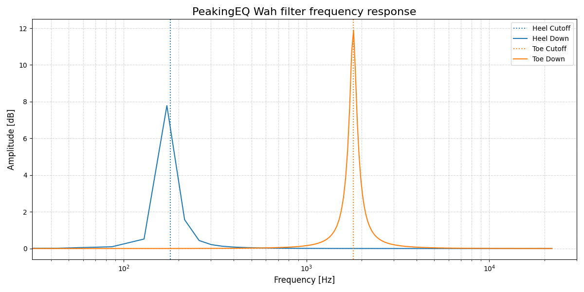
This doesn’t really seem to do the trick. At this point my suspicion is that this is because the peak is not high and narrow enough. Let’s redesign the filter with some different types.
PeakingEQ Filter
This experiment with the PeakingEQ filter is me fundamentally misunderstanding what it does.
I’m leaving it in here because it might be interesting for the reader to see where I went wrong.
For actual results skip to the Band-pass Filter section.
Let’s try a peaking EQ filter which should sound quite a bit more pronounced.
The PeakingEQ filter as given by the formula:
$$ H(s) = \frac{}{s^{2}+\frac{s}{AQ}+1} $$
$$ b_{0} = 1 + \alpha A $$
$$ b_{1} = -2cos\omega_{0} $$
$$ b_{2} = 1 - \alpha A $$
$$ a_{0} = 1 + \frac{\alpha}{A} $$
$$ a_{1} = -2cos\omega_{0} $$
$$ a_{2} = 1 - \frac{\alpha}{A} $$
Using the same definitions of $\alpha$ and $\omega_{0}$ as before.
 0def peakingEQ(cutoff,Q,dBgain,Fs=44100):
 1
 2    w0 = 2 * np.pi * cutoff/Fs
 3    alpha = np.sin(w0)/(2*Q)
 4
 5    A = 10**(dBgain/40)
 6
 7    b0 = 1 + alpha*A
 8    b1 = -2*np.cos(w0)
 9    b2 = 1 - alpha*A
10
11    a0 = 1 + alpha/A
12    a1 = b1
13    a2 = 1 - alpha/A
14
15    num = [b0, b1, b2]
16    den = [a0, a1, a2]
17
18    return {'cutoff':cutoff,'num':num,'den':den}
19
20Q=8
21dBgain = 12
22peaking_heel_down = peakingEQ(180, Q, dBgain)
23peaking_toe_down = peakingEQ(1800, Q, dBgain)
24
25w_peaking_heel, h_peaking_heel = signal.freqz(peaking_heel_down['num'], peaking_heel_down['den'], fs=44100)
26w_peaking_toe, h_peaking_toe = signal.freqz(peaking_toe_down['num'], peaking_toe_down['den'], fs=44100)
27
28fig3, ax3 = plt.subplots()
29ax3.set_title(f"PeakingEQ Wah filter frequency response")
30ax3.axvline(peaking_heel_down['cutoff'], color='C0', linestyle=':')
31ax3.semilogx(w_peaking_heel, 20 * np.log10(abs(h_peaking_heel)), 'C0', label="heel down")
32ax3.axvline(peaking_toe_down['cutoff'], color='C1', linestyle=':')
33ax3.semilogx(w_peaking_toe, 20 * np.log10(abs(h_peaking_toe)), 'C1', label="toe down")
34ax3.legend()
35ax3.set_ylabel("Amplitude [dB]")
36ax3.set_xlabel("Frequency [Hz]");
Let’s apply these filters to our sound sample
0from scipy.signal import filtfilt
1peaking_heel_down_signal = filtfilt(peaking_heel_down["num"], peaking_heel_down["den"], data.T[-1])
2Audio(peaking_heel_down_signal.T, rate=samplerate)
0peaking_toe_down_signal = filtfilt(peaking_toe_down["num"], peaking_toe_down["den"], data.T[-1])
1Audio(peaking_toe_down_signal.T, rate=samplerate)
0specgram2, (raw_peaking_spec, heel_peaking_spec, toe_peaking_spec) = plt.subplots(nrows=3)
1raw_peaking_spec.specgram(data.T[-1],Fs=samplerate, NFFT=1024);
2heel_peaking_spec.specgram(peaking_heel_down_signal,Fs=samplerate, NFFT=1024);
3toe_peaking_spec.specgram(peaking_toe_down_signal,Fs=samplerate, NFFT=1024);
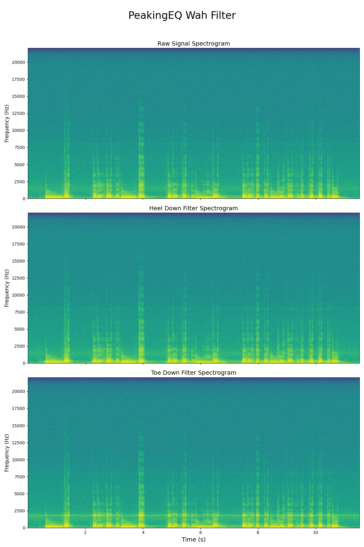
Band-Pass Filter
I made a mistake selecting the peakingEQ filter. This filter only boosts certain frequencies and doesn’t actually filter them i.e. the bottom of the frequency is at 0dB, where we need to have negative gain everywhere except for the passband. This means that I need to implement a band pass filter (BPF) instead. There’s 2 types in the cookbook: one with constant skirt gain and one with constant 0dB peak gain. We only want the wah to filter, not add any additional gain. Hence we use the constant 0dB peak gain BPF.
$$ H(s) = \frac{\frac{s}{Q}}{s^{2}+\frac{s}{Q}+1} $$
$$ b_{0} = \alpha $$
$$ b_{1} = 0 $$
$$ b_{2} = -\alpha $$
$$ a_{0} = 1 + \alpha $$
$$ a_{1} = -2cos\omega_{0} $$
$$ a_{2} = 1 - \alpha $$
Using the same definitions of $\alpha$ and $\omega_{0}$ as before.
 0def bandpassfilter(cutoff, Q, Fs=44100):
 1
 2    w0 = 2 * np.pi * cutoff/Fs
 3    alpha = np.sin(w0)/(2*Q)
 4
 5    b0 = alpha
 6    b1 = 0
 7    b2 = -1 * alpha
 8
 9    a0 = 1 + alpha
10    a1 = -2*np.cos(w0)
11    a2 = 1 - alpha
12
13    num = [b0, b1, b2]
14    den = [a0, a1, a2]
15
16    return {'cutoff': cutoff, 'num': num, 'den': den}
17
18
19Q = 8
20bandpass_heel_down = bandpassfilter(180, Q)
21bandpass_toe_down = bandpassfilter(1800, Q)
22
23w_bandpass_heel, h_bandpass_heel = signal.freqz(bandpass_heel_down['num'],
24                                                bandpass_heel_down['den'],
25                                                fs=44100)
26w_bandpass_toe, h_bandpass_toe = signal.freqz(bandpass_toe_down['num'],
27                                              bandpass_toe_down['den'],
28                                              fs=44100)
29
30fig4, ax4 = plt.subplots()
31ax4.set_title("Bandpass Wah filter frequency response")
32
33ax4.axvline(bandpass_heel_down['cutoff'], color='C0', linestyle=':')
34ax4.semilogx(w_bandpass_heel,
35             20 * np.log10(abs(h_bandpass_heel)),
36             'C0',
37             label="heel down")
38
39ax4.axvline(bandpass_toe_down['cutoff'], color='C1', linestyle=':')
40ax4.semilogx(w_bandpass_toe,
41             20 * np.log10(abs(h_bandpass_toe)),
42             'C1',
43             label="toe down")
44
45ax4.legend()
46ax4.set_ylabel("Amplitude [dB]")
47ax4.set_xlabel("Frequency [Hz]");

0bandpass_heel_down_signal = filtfilt(bandpass_heel_down["num"],
1                                     bandpass_heel_down["den"],
2                                     data.T[-1])
3Audio(bandpass_heel_down_signal.T, rate=samplerate)
0bandpass_toe_down_signal = filtfilt(bandpass_toe_down["num"],
1                                     bandpass_toe_down["den"],
2                                     data.T[-1])
3Audio(bandpass_toe_down_signal.T, rate=samplerate)
0specgram2, (raw_bandpass_spec, heel_bandpass_spec, toe_bandpass_spec) = plt.subplots(nrows=3)
1raw_bandpass_spec.specgram(data.T[-1],Fs=samplerate, NFFT=1024);
2heel_bandpass_spec.specgram(bandpass_heel_down_signal,Fs=samplerate, NFFT=1024);
3toe_bandpass_spec.specgram(bandpass_toe_down_signal,Fs=samplerate, NFFT=1024);

0
1sample_filtered = np.zeros(len(data.T[-1]))
2signal_in = data.T[-1]
3zi = signal.lfilter_zi(bandpass_toe_down['num'],bandpass_toe_down['den'])
4for i in range(len(data.T[-1])):
5    sample_filtered[i], zi = signal.lfilter(bandpass_toe_down['num'], bandpass_toe_down['den'], [signal_in[i]], zi=zi)
0specgram3, sample_filtered_spec = plt.subplots()
1sample_filtered_spec.specgram(sample_filtered,Fs=samplerate, NFFT=1024);
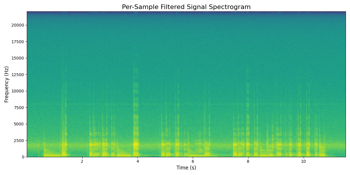
0Audio(sample_filtered, rate=samplerate)
This shows that I can do per-sample based filtering. Now we should adapt it so the filter varies between the two filters. I guess the first step here is introducing some normalization.
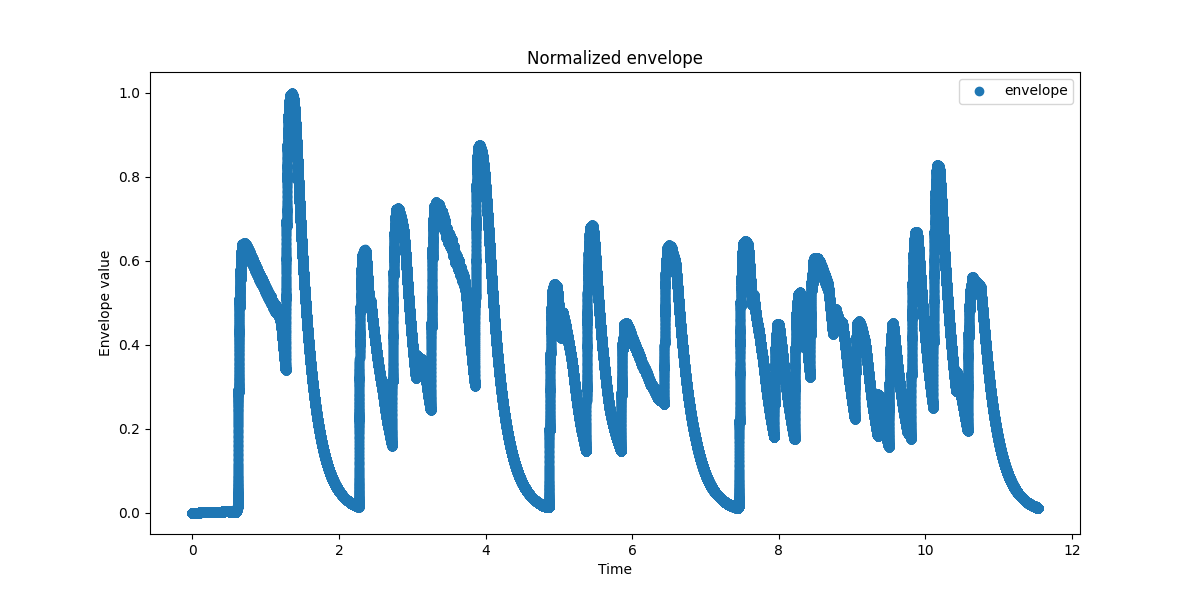
 0normalized_envelope = envelope / np.max(envelope)
 1
 2fig_env_norm, ax_env_norm = plt.subplots()
 3ax_env_norm.set_title("Normalized envelope")
 4
 5
 6ax_env_norm.plot(time, normalized_envelope, 'o', label="envelope")
 7
 8ax_env_norm.legend()
 9ax_env_norm.set_ylabel("Envelope value")
10ax_env_norm.set_xlabel("Time");
 0sample_envelope_filtered = np.zeros(len(data.T[-1]))
 1signal_in = data.T[-1]
 2# Always start in heel-down position.
 3zi = signal.lfilter_zi(bandpass_heel_down['num'],bandpass_heel_down['den'])
 4
 5freq_min = 180
 6freq_max = 1800
 7freq_range = freq_max - freq_min
 8
 9for i in range(len(data.T[-1])):
10    freq = freq_min + normalized_envelope[i] * freq_range
11    env_filt = bandpassfilter(freq,Q)
12    sample_envelope_filtered[i], zi = signal.lfilter(env_filt['num'], env_filt['den'], [signal_in[i]], zi=zi)
0specgram4, sample_env_filtered_spec = plt.subplots()
1sample_env_filtered_spec.specgram(sample_envelope_filtered,Fs=samplerate, NFFT=1024);
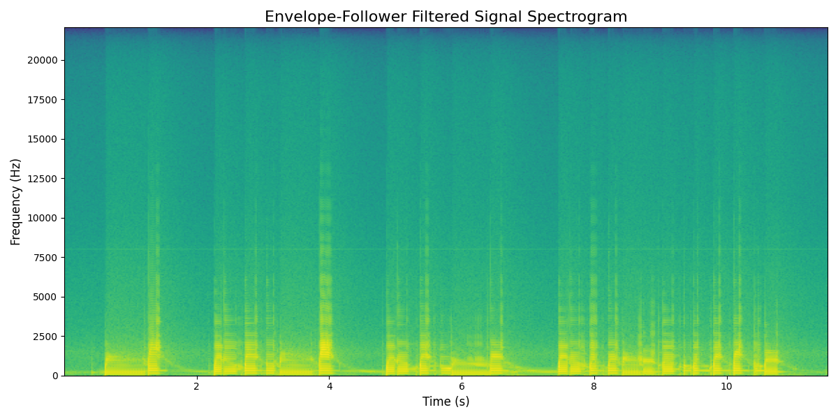
0Audio(sample_envelope_filtered, rate=samplerate)
Conclusion
I think I’ve got the basis now for an envelope filter that I can continue to work on. The next steps are playing around some more with the parameters, figuring out what the topology of an actual effect would be (do we need additional effects to make it sound as good as possible?) and converting this code to C++ using JUCE to make an actual effect out of it.